A few days ago I was chatting with a fellow colleague (Jon Parker, great Houdini Artist) about magnetic fields. So I decided to create a little OTL to generate a vector field starting from a pole cloud distribution and share the workflow, since it's really simple to implement and the results are great. I am not sure (actually I highly doubt) that the following implementation is physically correct in any way, I just wanted to have a way to quickly create a magnetic-looking vector field.
I generally use Wrangle nodes pretty much for everything since it's very quick to create, initialize attributes and modify their value with just a few lines of code. Feel free to use VOP nodes if you prefer a node-based approach.
For what concerns Volumes, I generally prefer to use VDB (when I am not forced to use Houdini Volumes). VDB have an optimized memory structure that allow a very fast access to voxels data, plus they are sparse so they have a lower memory foot print compared to Houdini Volumes. They are slightly more tricky to use, but the reward is huge in terms of speed and memory.
Let's start simple. Two points with a "f@pole" attribute that can be either +1 or -1.

For mere visualization purpose I created a little setup where a sphere is copied (copy SOP) to each point ...

.. the sphere is RED if the pole is negative, and GREEN if the pole is positive (using a copy SOP and the stamp expression function).

Using a wrangle node and the stamp function in one of the parameters I can select the color of each sphere based on f@pole attribute.

EDIT : I was completely unaware of chv ( ... ) vex command, which allows to read directly a vector parameter from the UI (thank you anonymous poster !!). Which means that the lines above can be written, much more elegantly, this way :
vector negcol = chv ("negativecol");
vector poscol = chv ("positivecol");
... your setup should now look more or less like this.

It's now time to create the Volume that will contain our vector field.
Let's create a VDB node, make sure to give the field a name (I used "magneticfield"), and set it to be a vector field.
 This will create an empty VDB volume. By default a VDB volume is dimensionless. Why ? Cause VDB is a sparse volume, meaning that it exists only where we want to. Consequently we need to "activate" the VDB in the regions of space where we need it, before actually 'filling' it.
 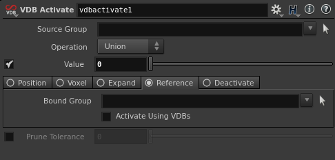 In order to do that, we use "VDB_activate" SOP which allows to use geometry to activate the region.
  In this case I am using a bounding box, with some padding, generated directly by my point cloud.
This is what the node graph should look like roughly.
NOTE: don't forget to enable "Pack Geometry before Copying" in the Copy SOP, under Stamp section (later, when we'll use thousands of points, this option will make a huge difference).

And the viewport (note the empty VDB defined by the bounding box surrounding the poles):

There's one more step we should follow before starting to write our Volume Wrangle node. At the moment, we wouldn't be able to visualize the content of the Vector VDB cause of the nature of a vector field. For this purpose we can use the Volume Trail node. This node will sample the vector field in the points specified by the First Input , and draw curves following the vector volume connected in the Second Input.
 I used the previously created bounding box to generate a Fog Volume, and scatter points within it. These will be the sample points used by the Trail SOP.
 And this is what the graph should look like. Note that the sample points go in the input 1 of the Volume Trail SOP.
Now, we can't see any trail cause the vector field is empty. Let's test if it works filling the volume with a constant vector.

Your viewport should now look like this.
Horizontal lines, matching the horizontal vector {1.0 , 0.0 , 0.0 }.

Now we have a good environment that will allow us to visualize and debug our code.
Let's now discuss how to calculate the magnetic field resulting by the 2 poles , for each voxel in the VDB grid.

Let's calculate the magnetic field generated by the poles p1 and p2 at the position v@P (the dark grey voxel visible in the picture above).
That Voxel will feel the negative influence of p1 (meaning , will be repelled from p1) and the positive influence of p2 (meaning, will be attracted towards p2). If we calculate the vector distance between the voxel and each pole position, of course we obtain a vector that is very small when the voxel is close to the point, and very big when it's far. We want the opposite. That's why, in our calculation we use the inverse of the distance from each pole, as a multiplier of the (normalized) distance vector. This way, the closer we are to the pole, the stronger is the attraction or repulsion as you can see from the function plot below.

d is red (no good, cause it gets bigger and bigger with the distance)
1/d is green (good cause it big close to the pole, and smaller and smaller far from the pole).
This was the trickiest part. The rest is pretty simple.
All we need to do is to store in each voxel the sum of all the normalized distance from each pole position, multiplied by the pole attribute ( to make sure the contributing vector is repelling or attracting depending on the pole ) and multiplied again by the inverse of the distance, as explained before.
The pseudo code is the following:
- For each Voxel position v@P
- initialize a vector called VectorField = { 0 , 0 , 0 }
- iterate through all the points (pi) in a certain radius from v@P
- import the pole attribute of the point, pole
- find the vector d between pi and v@P
- find the normalized (nd) and magnitude (md) of vector d
- add nd , multiplied by pole, and by the inverse of the distance md to VectorField
- the magnetic field v@magneticfield in the voxel v@P is set to VectorField
Let's create a Volume Wrangle, and connect the Input 1 to the VDB volume , and the input 2 to the merge node containing the 2 points with the "pole" attribute.

Converting the pseudo code in VEX is probably easier than writing the pseudo code itself.

Now this is what the view port should look like:

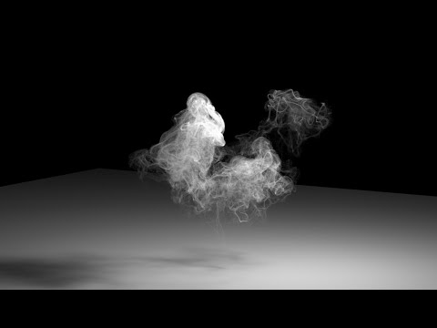
Now we can replace the boring 2 poles setup with something more attractive.
How about ... simulating the magnetic field on the surface of the sun ?

This picture I downloaded from Google Image is a good reference.
In order to recreate that look, all we need to do is scatter points on a sphere (about 2k), randomly assign f@pole to -1 or 1 and feed it into the simple setup we just created.

I find this pretty cool ! :)
Ok, I guess that's it.
If you like this tutorial, or found a better way to achieve the same result, please don't hesitate to comment.
Thank you for reading !
Since you read the whole article you definitely deserve the hip file.
It's better to use the inverse of the square of the distance, instead of the inverse of the distance. This will definitely give better results and less interference in the voxels far from poles.
Thanks to Jon Parker for this suggestion.
[ EDITED in 2015 ]
[ EDITED in 2015 ]
ADVECT PARTICLES ALONG THE CURVES
Many people asked me this question:
Great job with the lines, but ... what now ?? For instance, how do I advect particles along those lines ?
Ok this is what I would do.
First off I assume you are creating some kind of Sun Flare FX, so I assume you've got your sun surface from which you're generating your magnetic arcs.
I'll write here broad strokes, without really going into details for now and see if that works:
- find a way to create a direction vector on the lines (one way could be using a PolyFrame SOP). Let's call this v@linedir , and find a way to orient this path so that it goes in the dir you want (like from the positive to the negative or the other way around).
- emit particles from the surface of the sun in some POP network
- using a POP Wrangle open a point cloud (pcopen / pcfind) on the curves, sample v@linedir attribute (using pcfilter or pcimport in a for loop ...) to return an average direction (lets call it magv) and add it to the particles velocity (v@v += magv).
- optionally use the distance from the sun to modulate magv length using a ramp.